Anyone that has ever undertaken a complex energy efficiency project in their building knows that it often takes longer to get the utility incentive than to complete the project. One reason? The procedures to verify the savings are complex, manual and subject to layers of review.
This is a problem if we want energy efficiency to scale up. Not only should the customer experience be better, but we literally don’t have enough engineers in America to verify the anticipated growth in energy efficiency projects. This is why leaders in energy efficiency and measurement and verification have been excited to study automated techniques based on smart meter data.
The most exciting and large scale study (pdf) was conducted over the last year at Lawrence Berkeley National Labs (LBNL) with funding from the United States Department of Energy. The objective was simple: test numerous commercial and academic models on a large number of buildings to see how well they could predict each building’s future baseline energy use. If the models are accurate enough, then utility programs might automatically calculate savings as the difference between meter readings and that future baseline.
LBNL tested two essential and complementary metrics of statistical model accuracy–one that reads the total difference between model predicted energy use and actual metered energy use, and another that reads the model’s ability to predict the overall load shape reflected in the data. The chart below summarizes the study results of 7 models developed by commercial entities such as Gridium (our model is referenced as “M3” in the report), and 3 academic models deployed across 537 buildings.
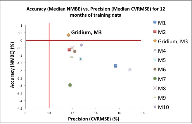
Gridium’s model is closest to optimal, across 10 tested models. Details below. Chart from the LBNL study, adapted for clarity.
Quoting LBNL, “This is promising for the industry.”
In general, the models tested were able to predict whole-building energy use with a high degree of accuracy and minimal bias. This is encouraging; in the first major test of these models, most models performed well enough to pave the path toward a future of automated M&V.
We’re extremely proud of Gridium’s results. As depicted above and showing the relationship between bias (accuracy) and error (precision), Gridium’s “M3” results are the most optimal. The study tested the models 12 different ways, taking each median measurement across each training period individually, and Gridium’s model is in first place 7 times and second place 5 times. When you use Gridium software for M&V, you know you are getting best in class performance.
This LBNL assessment is validation that smart meter data analytics are accurate, and that there’s real potential in adopting them. There’s still a lot of work to do before you’ll see these approaches in utility programs, but you can access the leading tools in our suite of energy management software.
For those who want to dig a little deeper, let’s dive a bit more into the study.
How did LBNL test these models?
15 minute whole-building electric meter interval data was gathered for 537 commercial buildings across the United States. Data for each building was divided into hypothetical training periods of different lengths (industry-standard 12 months as well as 9 months, 6 months, and 3 months) and prediction periods of 12 months. Meter data from the prediction period was “hidden” from the model. The trained model would then forecast the building’s load throughout the prediction period, and this prediction was then compared to the actual meter data that had been hidden.
Two performance metrics were used to quantify the model’s predictive accuracy.
Firstly, the total difference between model predicted use and actual metered use was measured by the normalized mean bias error (NMBE). This is a reading of accuracy. NMBE is the amount by which the model is consistently wrong: a negative NMBE means the model consistently underestimates demand. A sports analogy helps- having a large negative bias is like being handicapped as though you are a better golfer than you truly are. This means you have to overcome this additional handicap just to get back to even. If the purpose is to assess savings, a large negative bias puts your building in an artificially deeper hole because you have to overcome the bias first before any savings can be accurately credited to your building.
Secondly, the model’s ability to predict your building’s overall load shape was measured by the coefficient of variation of the root mean squared error (CV(RMSE)). This is a reading of precision. It measures the ability of each model to predict a 15 minute reading, 12 months in advance! It’s a special challenge, but relevant for capturing demand savings, time of use savings, and is the main measure in the influential ASHRAE Guideline 14.
NC State University provides the best explanation of the relationship between accuracy and precision: “…imagine a basketball player shooting baskets. If the player shoots with accuracy, his aim will always take the ball close to or into the basket. If the player shoots with precision, his aim will always take the ball to the same location which may or may not be close to the basket. A good player will be both accurate and precise by shooting the ball the same way each time and each time making it in the basket.”
While we’re proud of Gridium’s results, we’re even more proud that the techniques we have advocated for performed so well across the industry. This means that policy makers can take an automated path without relying too much on Gridium’s algorithms. Some of the models have even been open sourced!
However, we also want to demonstrate that the major comparative split in the study is between a handful of accurate models and handful of relatively less accurate models. There are models whose accuracy really shines and models that, as LBNL describes it, are “outliers.” For the standard case of 12 months of training data, these outliers include M1, M4, and M7. For non-standard training data periods of 9, 6, and 3 months, M9 joins the cluster of M1, M4, and M7 with relatively higher error readings. If you are exploring energy software tools for M&V, you’ll obviously want to purchase a tool in the better cluster.
A detailed review of each model across each training period length can be found on pages 14 through 18 of the LBNL report. A final editorial note. Our parents taught us to be polite, so we aren’t naming the outlier models, but they are named in the report.
